(The content on these pages may be freely used for educational, noncommercial purposes provided appropriate references are provided. Commericial users are kindly asked to contact me first. Be aware that in any case, they come with no warantee: use at your own risk!)
Terminal velocity in fluid
This simple machine demonstrates that a viscous suspension (applesauce) suspended in water has a pretty low terminal velocity. After it reaches terminal velocity, it travels at a constant speed. This is well modeled by the transport equation.
The heat equation
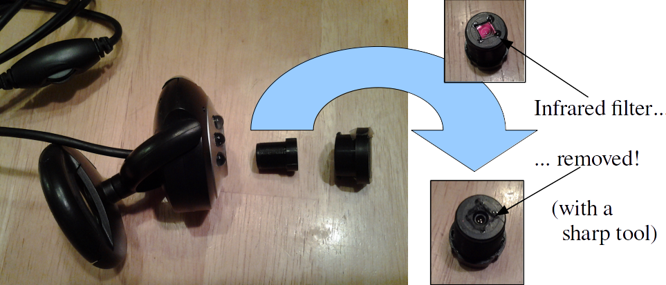 Any demonstration involving the heat equation should involve fire. But how to easily measure the temperature of something hot? Simple: make use of the fact that digital cameras are already sensitive to the infrared emissions radiated by hot objects. They usually have a protective lens to filter out infrared, but it's easy to take an inexpensive webcam and remove the filter. Then you have an infrared webcam!
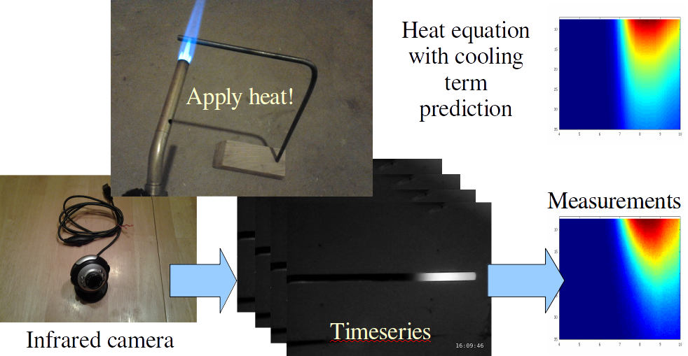
Then, take a metal rod and heat it with a torch so that it's glowing hot, and snap a sequence of pictures of it with the infrared webcam as it cools down. If you take enough pictures, you can compare the temperature as a function of time with the heat equation (you need to account for lateral heat loss, which is an extra loss term). The fit between theory and practice is not too bad!
Shive wave machine
Torsional waves on a wire can have very low propagation speeds -- they're so slow that you can see them moving. John Shive invented a simple machine to demonstrate these waves to his students. It's pretty easy to build a tabletop version yourself with a few parts from a hardware store. Then you can see wave propagation and standing waves quite clearly.
Lissajous figure maker
An excellent example of parametric curves can be found in the example of a Lissajous figure. These can be generated in a variety of ways, perhaps most commonly using the X and Y inputs of an oscilloscope. However, that's kind of high-tech. In the past, they have been generated mechanically, often involving vibrating strings. Most vibrating strings don't move very much, so some old experimental descriptions require looking at the Lissajous figures through a magnifier. A much simpler way to generate them requires two mirrors mounted on rotating axes at right angles to one another. A beam of light can be directed between the mirrors to project a Lissajous figure on a screen.
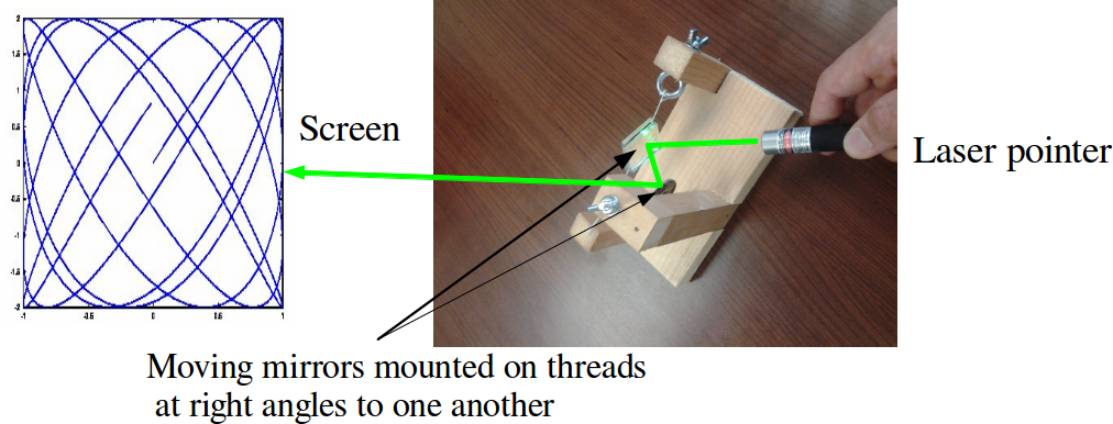 To make something suitable to show in a classroom setting, I made a frame that held two strings at right angles to one another. The strings are hung from screw eyes with wing nuts so that the tension can be adjusted. (This is inspired by the mirror galvanometer.) To each string, I attached two small mirrors (about 1" x 1" square) back-to-back with a little tape. I tried attaching one mirror to each string, but found that the assembly wasn't very well balanced -- two identical mirrors are much better balanced. The mirrors are aligned so that a laser beam can bounce off both mirrors before being projected onto a screen (usually the wall).
L'Hospital's rule demonstrator
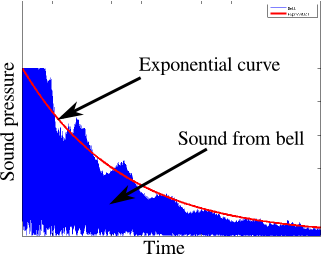
Which function decays faster: an exponential decay or a power law decay? This question is one of the things that L'Hospital's rule makes short work of in class, but can this mathematical question be answered with an experiment? Yes! In acoustics, sounds often decay sharply as energy is dissipated. For instance, the sound pressure of a bell as it rings tends to follow an exponential decay. Exponential decays also can be generated easily with a resistor-capacitor circuit.
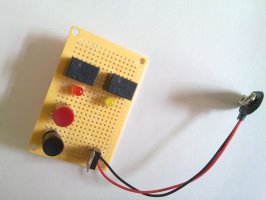
 Power law decay is a little more subtle, but it's pretty well-known that sound pressure decays according to an inverse square law. This demonstration pits power-law decay coming from moving away from a sound source against the exponential decay coming from a resistor-capacitor circuit. In order to be easily moved, the circuit has to be small. Here is the circuit diagram. I built mine so that the separate functional components are easy to see and debug, should something go wrong.
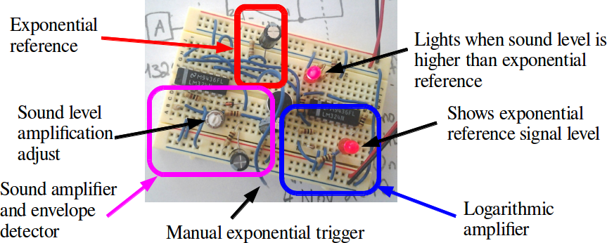 L'Hospital's rule is about limits of ratios, so it's proper to have the circuit manipulate the ratio of the two signals. However, circuits that compute ratios are a bit tricky. It's much easier to compute logarithms and subtract, which is what this circuit does. The input stage to the circuit consists of a resistor-capacitor timer (triggered by a switch, and displayed with an LED) and a microphone audio amplifier. These are fed into a pair of logarithmic amplifiers. These feed into a difference amplifier, working as a comparator. The comparator drives the output LED.
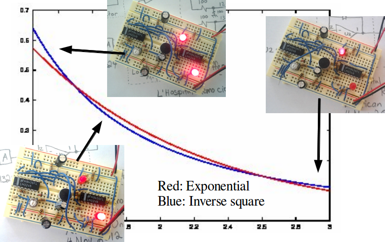 I found that the circuit was a little tempermental after it was built. This is mostly because of the fact that the logarithmic amplifiers can have pretty large gain because they're nonlinear. Once everything is adjusted correctly, the circuit does a nice job. If you're going to perform the experiment in front of an audience, you should practice until you have the technique mastered. First, you need a constant sound output. There are various ways to get this, for instance playing a sound file on your cell phone or laptop. (I like to use gst-launch utility on Linux to generate a tone.) However, it's also workable to whistle a clear, stable note, although this takes practice. Once you have the sound source working, here's what to do:
- Place the circuit on the table,
- Start the sound source right near the microphone, (the sound level LED will light)
- Push the trigger button, (the sound level LED will extinguish, but the exponential LED will light)
- Slowly move the sound source away from the microphone...
- Until the sound level LED lights again.
Clepsydra (water clock)
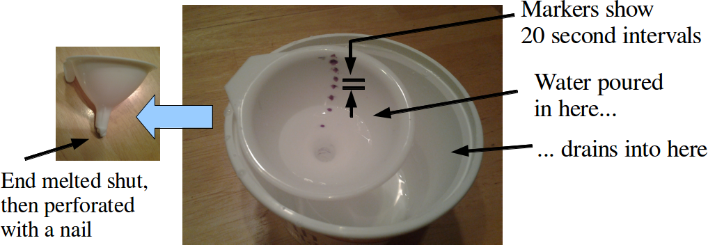 Here's a quick little demonstration that highlights some simple, old ideas. Dripping water happens to be a good timekeeper, and is a good introduction to related rates problems. It's pretty easy to make. Take a plastic funnel and melt the end shut with a candle. Then puncture the now sealed end of the funnel with a nail to make a small hole. Fill the funnel up with water, start a stopwatch, and mark off where the water level is (use a grease pencil) at some fixed time interval. It'll take a little trial and error to figure out what that interval should be. If the funnel drains too fast, seal the end again and make a smaller hole.
What do you do with this once you have it? Hand a student a stopwatch and have another student read off when the water level crosses the markers -- they're usually pretty surprised that the time intervals get farther apart as the water level goes down. Then, derive the rate of change of water level as a function of volume -- it's not a bad match if you use the volume of a cone.
Sound Card Sonar
I realized in preparation for the topological imaging experiments that there is little additional overhead required to apply traditional signal processing chains to the data collected. In this case, both the transmit and receive hardware is simply an off-the-shelf laptop and GNU Octave.
Image formation
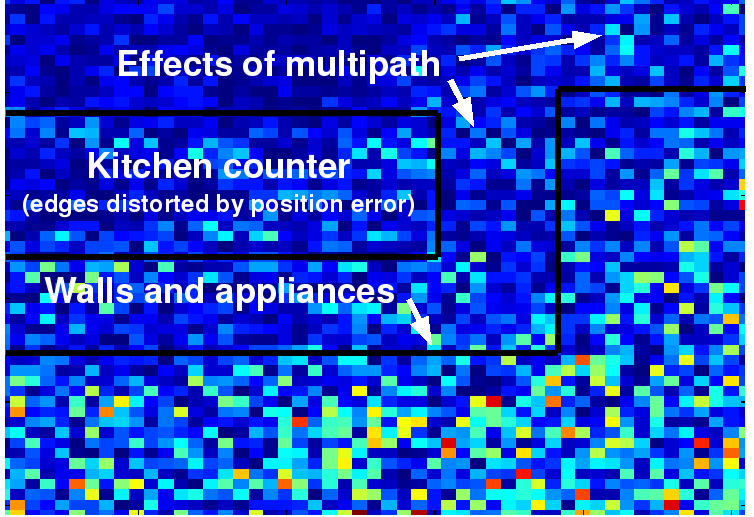
It is straightforward to write simple, non-optimized sonar image formation software. I have typically used my smartphone to act as the transmitter, by playing a carefully constructed audio file that contains a number of chirped pulses. I receive the echos through the microphone on my laptop computer, perform some noise equalization using the freely-available program Audacity, and then pass the data over to my processing chain in Octave.
The resulting imagery can sometimes be a bit difficult to interpret, especially since interesting environments are rarely two-dimensional, as typical image formation algorithms expect. The wavelength of sound is also physically quite long, so the effects of diffraction and reflection are quite pronounced, and produce noticeable bright spots at corners of a room. As far as I know, the only other instance of this kind of thing is here, and sadly it seems like it hasn't been updated in a while.
Real-time audio tools
Working with acoustic data is very convenient because the experimenter can hear many problems instantly. In addition, since the rise of powerful multimedia frameworks such as GStreamer and python bindings for them, platform-independent, custom audio test equipment is very easy to construct. So I have availed myself of the opportunity and written a small collection of tools that the typical sonar engineer wants to have.
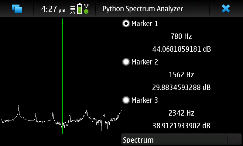
For
instance, I have written an audio spectrum analyzer that can display
the log magnitude spectrum, autocorrelation, or other desired
functions of the received audio. Since the tool is written in
platform-independent python, it runs on my Linux laptop (based on the
x86 architecture) and my Nokia n900 smartphone (based on an ARM
processor) with no changes to the code.
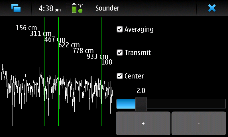
Sonar
engineers are often in need of accurate ranging information, so I
wrote a simple channel sounder. It emits a stream of brief clicks and
then integrates the result. Typically, targets of high acoustic
reflectivity (walls, for instance) appear as spikes on the display.
Sadly, the user interface isn't as pretty as the
iPhone
sounder, but mine is platform-independent and interpreted, so it
is extremely easy to modify to fit my needs.
Synthetic aperture sonar
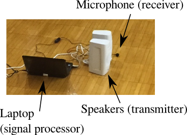 With very little equipment, you can run a real-time sonar system! It requires
- A laptop running Linux, with Python GTK and GStreamer libraries
- A set of speakers -- the bigger the better, with good high-frequency (tweeter) response
- A microphone, again with good high-frequency response
- A waveform to transmit, such as squeak.wav (a low-ultrasound chirp), squeaks.wav (a chirp train), or clicks.wav (an audible click train).
- And some processing software, such as this bundle. The range-doppler sounder takes a lot more CPU horsepower, so it might have trouble staying real-time.
Opportunistic imaging
System requirements and installation
- Python 2.5 or newer
- GTK and python bindings
- GStreamer and python bindings
- the Python numpy and scipy libraries
- Python WAV file import (should be standard)
- python-numpy
- python-scipy
Demonstrations using acoustic sounders
This experiment demonstrates the signal space embedding theorem (see "Topological localization via signals of opportunity") for acoustic signals. The basic idea is that a collection of simple transmitters (special hardware used, but it's not crucial) emit signals received by a single receiver (laptop computer sound card). In order to provide some discrimination of which received signal corresponds to which transmitter, the transmitters emit short pulses, one after the other. The transmit sequence is enforced by a simple one-wire handshake. As it happens, the software framework for receiving supplied below loses synchronization frequently, so we can only identify transmitters up to a cyclic permutation. Even in spite of this, the signal embedding theorem guarantees unique signal response for each receiver location if enough transmitters are present. Downloadable items for conducting the experiment: ZIP file here
- rx_tdma_chirp.py: runs the receive and decode process on the receiver laptop. This produces an output text file in which each row corresponds to a measurement.
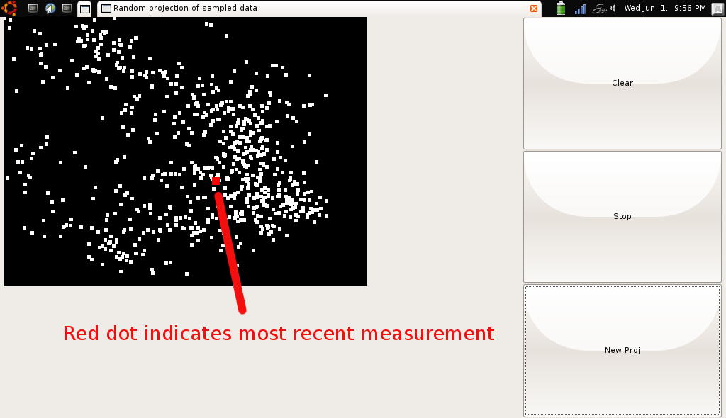
- projectPoints.py: a real-time display of points projected from high dimensional Euclidean space to the plane. It uses the output of rx_tdma_chirp as its input.
- Schematic and directions for the acoustic sounder
- The sounder contains a PIC16F88 microcontroller. Here is the source code for it.
 Step-by-step instructions for conducting the experiment:
- Apply power to each individual sounder
- Connect the signaling wires between each sounder
- Start the sounders emitting chirps by briefly grounding one of the signaling wires on one of the sounder. Reattach it before the active transmitter returns to the one you started.
- Start the receive thread using the command "rx_tdma_chirp -m level -t number of transmitters"
- Start the display thread using the command "projectPoints number of transmitters out.txt"
Software to work with anything that can play sound files
Instead of using special hardware for transmitting signals, anything that can play a sound file can be used. Matched filters can be used to discriminate between the different choices of signals, though as in the previous experiment, several transmitters can emit the same signal. Rather than conducting the experiment in real time, this experiment collects data on request for offline processing. This can enable more experiments that are more carefully controlled.
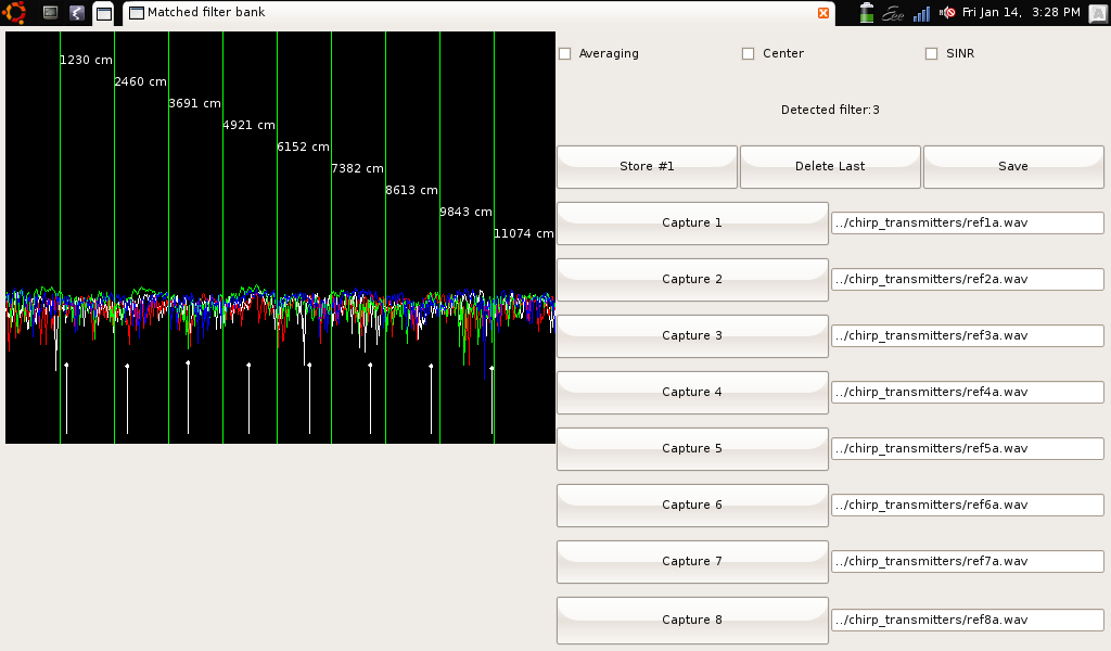
- matfilter.py implements a simple bank of 8 matched filters. Each filter can have a reference signal taken from a recording taken just before the experiment (while the program is running), or from an uncompressed WAV file.
- Here are several chirp files in WAV and MP3 format, though you could use anything, really. These particular ones have mutual isolation of better than 10 dB.
 Step-by-step instructions for conducting the experiment:
- Start up the matched filter program
- Load each reference file, either by playing a clip and pressing the Capture button, or by typing in a filename of a WAV file containing the reference. Press Enter after each filename to trigger it to load.
- Set up and activate the transmitters
- Once everything is in order, press the Store button to take data
- Repeat collection of data (pressing the Store button for each datapoint). If you make a mistake, you can delete datapoints.
- Once complete, press the Save button to save your datafile.
Here is some sample data, and at right is a screenshot of the program in action.
Imaging with wireless access points
Thanks goes out to Daniel Muellner and Mikael Vejdemo-Johansson for the scripts used in this demo!
Instead of acoustic sounders, you can use wireless access points to generate the ambient signals for localization. Here are a few scripts that read data (under Linux or Mac OS) from a wireless card and format it appropriately for projectPoints.py.
- ssidcollect_linux.py: collects the ethernet (MAC) addresses of wireless access points in range and their signal strengths. On my computer at least, it requires you to be connected to one of them in order to get data. Your mileage may vary. I ran this on my Nokia n900 phone using a slightly modified script ssidcollect_maemo.py, and a Mac OS version: ssidcollect_macos.py.
- ssidaccumulate.py: formats the output of ssidcollect_linux.py into a CSV file, similar to the data from the acoustic experiments above.
Step-by-step instructions for conducting the experiment:
- Connect your computer to a wireless network (may be optional depending on your wireless drivers)
- Make sure the collection works: "ssidcollect_os.py". You may have to use "sudo" to run this depending on your system. Press Control-C or equivalent to stop the collection.
- Acquire data "ssidcollect_os.py > data.log"
- Reformat it into a CSV file for later useage "ssidaccumulate.py < data.log > data.csv"
Asynchronous circuits
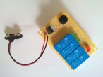
 Asynchronous circuits are very easy to see when the logic gates aren't very fast. Although one could use delay circuits to show this with transistorized electronics, it is trivial to make slow asynchronous circuits using relays. Here are the schematics for two example circuits: a Glitch generator and an RS flip-flop.
Thanks goes out to Daniel Muellner and Mikael Vejdemo-Johansson for the scripts used in this demo!
Instead of acoustic sounders, you can use wireless access points to generate the ambient signals for localization. Here are a few scripts that read data (under Linux or Mac OS) from a wireless card and format it appropriately for projectPoints.py.
- ssidcollect_linux.py: collects the ethernet (MAC) addresses of wireless access points in range and their signal strengths. On my computer at least, it requires you to be connected to one of them in order to get data. Your mileage may vary. I ran this on my Nokia n900 phone using a slightly modified script ssidcollect_maemo.py, and a Mac OS version: ssidcollect_macos.py.
- ssidaccumulate.py: formats the output of ssidcollect_linux.py into a CSV file, similar to the data from the acoustic experiments above.
- Connect your computer to a wireless network (may be optional depending on your wireless drivers)
- Make sure the collection works: "ssidcollect_os.py". You may have to use "sudo" to run this depending on your system. Press Control-C or equivalent to stop the collection.
- Acquire data "ssidcollect_os.py > data.log"
- Reformat it into a CSV file for later useage "ssidaccumulate.py < data.log > data.csv"
Asynchronous circuits
Asynchronous circuits are very easy to see when the logic gates aren't very fast. Although one could use delay circuits to show this with transistorized electronics, it is trivial to make slow asynchronous circuits using relays. Here are the schematics for two example circuits: a Glitch generator and an RS flip-flop.